

TITARL Tutorial
1. Introduction
 What is TITARL?
TITARL is a Data Mining algorithm that is able to extract Temporal Association Rules from Symbolic Time Sequences and Scalar Time Series.
What is a symbolic time sequences or a scalar time series?
A symbolic time sequences is a record (i.e. a set) of symbolic events. A symbolic event is a symbol and a timestamp. A scalar time series is mapping from every timestamp to a scalar value.
The figure 1 shows an example of symbolic time sequences and scalar time series.
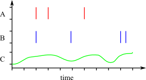
Fig.1: Example of symbolic time sequences and scalar time series.
In this figure, A and B are two symbolic time sequences. You can see three events of symbol (or type) A. The C is a scalar time series. You can see the value of C changing over time.
Symbolic time sequences and scalar time series are a powerful way to represent state and history real world systems. For example, Symbolic/scalar time sequences can describe:
- The page request made to an internet website (Every page request is a symbolic event).
- A financial market (The market value is represented as a scalar time series, and markets events are represented as symbolic time sequences).
- The physiological signs of patients in hospitals (The vital signs are a scalar time series, while the drug input and physician actions are symbolic time sequences).
- The transaction of a client in a shop (Each transaction is a symbolic event).
- The incidents and repairs of a ship or a plane (Each maintenance operation and each flight are a symbolic event).
What is a temporal association rules?
A temporal association rules is type of pattern that describes relations between objects with a temporal aspect (like a symbolic time sequences or a scalar time series). Let's start with an example of (non-temporal) association rule.
A simple example of (popular and inaccurate) association rule is: If a man buys diapers, then he will also buy beers.
This last rule does not have any temporal information. A simple example of temporal association rule is: If a man buys diapers at night, and if he did not buy beers over the last two days, then he will also buy beers with the diapers. This second rule includes some temporal information. Therefore, this rule will be called a temporal association rule.
The goal of TITARL is to find the most interesting temporal association rules in a symbolic/scalar time sequences. Such association rules can be used to understand the system they describe. They can also be used to forecast what will happens to this system in the future. This tutorial explains didactically how does the TITARL algorithm works.
And, what is the real use of a Temporal Data Mining algorithm like
TITARL?
Suppose a patient in an hospital. The patient is equipped with sensors that track his vital signs (e.g. the hearth rate or the respiratory rate). Those sensors can alert medical staffs if the patients is becoming unstable(e.g. the patient starts to breath too slowly).
If we have a large set of record of those sensors activities, the TITARL algorithm can be used to extract temporal association rules between those vital signs. The extracted rules will express the correlation between the vital signs of the patients and the eventual upcoming of instabilities of this patient. Next, those temporal rules can be analyzes to help the understanding of how the body of a patient works.
We can go further: Those temporal rules can by applied in real time so they can alert medical staffs event BEFORE patients become unstable. In this case, the physicians can act on patients before the patients' lives are threaten, and therefore, increase their chance of successful recovery.
The main use of TITARL is to extract rules in order to understand complex systems. Those rules can also be used to forecast/predict the future state of a system. TITARL rules can also be used to compare related systems : A system might fits certain rules while another one might not. Finally, TITARL rules can be used for temporal planning. Example of planning with TITARL rules has been presented in [Learning Temporal Association Rules on Symbolic Time Sequences - Guillame-Bert et Al.] and [Planning with Inaccurate Temporal Rules et Al.]. Before explaining TITARL, I will describe more precisely what are the temporal association rules that TITARL is able to extract:
2. The TITARL rules (or TITARs)
Like any association rule, a TITARL rule is composed of two parts: The condition (or the body), and the conclusion (or the head). When the condition of the rule becomes true, the rule is "activated", and it makes a prediction based on its conclusion (or head).
A very simple example of TITARL rule is:
Rule 1: If there is an event A at time t, then there will be an event of time B a time t+5. This rule is able to forecast events of type B based on events of type A. This rule can be written as : A[t] → B[t+5]. In this example, "A at time t" is the condition (or body) of the rule, and "B at time t+5" is the conclusion (or head).
The head of the rule is composed of two elements: The symbol to predict, and a temporal constraint for this symbol. In the previous example, the temporal constraint of the head is "t+5".
Because real world applications have a lot of uncertainty, this type of rule usually does not perform well. To solve this problem, TITARL rules can express uncertainty. More precisely, TITARL considers two types of uncertainty.
2.1 The confidence of the rule
The confidence of a rule expresses the confidence we can have in the predictions made by a rule. Titarl expresses confidence with a probability. An example of rule with a confidence is:
Rule 2: If there is an event A at time t, then there is 50% chance to have an event of time B a time t+5. In other words, there is 50% chance to have an event of type B exactly five seconds (if the time is expressed in seconds) after an event of type A. This type of rule is more flexible, and is generally more suited to describe real world systems. This new rule can be written as : A[t] → B[t+5] 50%
2.2 The temporal accuracy
Because time if generally considered to be continuous (or highly discretized), it is generally impossible to predict exactly when something will happen. To solve this issue, TITARL rules can express temporal inaccuracy. An example of rule with temporal inaccuracy is:
Rule 3: If there is an event A at time t, then there will be an event of type B between time t+5 and time t+10. In other words, this rule does not tell exactly when the event of type B will be, but it gives an approximation of its temporal location. This new rule can be written as : A[t] → [t+5,t+10]
Those two type of uncertainty can be combined together. An example of rule with temporal inaccuracy AND confidence is:
Rule 4: If there is an event A at time t, then there is 50% chance to have an event of type B between time t+5 and time t+10. This new rule can be written as : A[t] → B[t+5,t+10] 50%
The bodies of all those rules are always composed of the same condition: The detection of an event of type A. Rules with this type of condition (only one element) are called "Unit rules".
Such simple rules are not always powerful enough to describe a system. To solve this problem, TITARL is able to deal with more complex rules. Here are some example of complex rules:
Rule 5: If there is an event A at time t, and if there is an event of type B between [t-5, and t+5], then there is 50% chance to be an event of type C between time t+5 and time t+10.
orRule 6: If there is an event A at time t, and if there is an event of type B between [t-5, and t+5], and if there is an event of type C from 2 to 3 seconds before B, then there is 70% chance to be an event of type D between time t+1 and time t+3.
Rules 5 and 6 are rules with temporal constraints in the body.
As you can see, complex rules become hard to explain literally. To solve this problem, we developed a graphical notation for TITARL rules. The fig. 2 shows the graphical notation for all the example of rules we have presented until now.
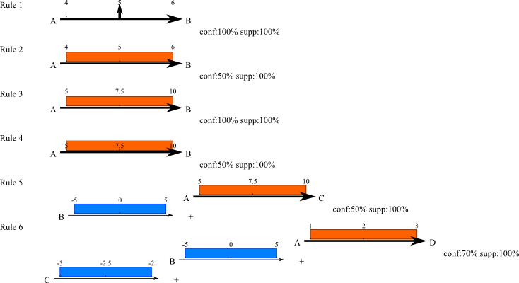
Fig.2 : Example of TITARL rules.
The rules can be seen as "trees of temporal conditions". In the previous examples, the conditions are always a tests of existence of an event in a given range of time (i.e. testing if there is an event of a given type in a given range of time). TITARL rules can also been condition on value of a time series. For example:
Rule 7: If there is an event A at time t, and if the value of the time series E at time t is lower than 0.5, then there is 50% chance to have an event of time B between t + 5 and t + 6.
TITARL rules can also express negation. For example:
Rule 8: If there is an event A at time t, and if there is no event of type B between t-2 and t+2, then there is 50% chance to have an event of time B between t + 5 and t + 6.
Until now, all the temporal constraints of the head of the rule were intervals. TITARL allows head (and body) temporal constraints to be non-connected sub-set of ℝ. An example of rule with non-connected temporal constraint is:
Rule 9: If there is an event A at time t, then there is 90% chance to have an event of time B either between t + 5 and t + 6, or between t+10 and t+10.
Until now, the temporal location of the prediction were uniformly distributed. For example, if a rule predicts an event of type B between 5 and 7, the probability for this event to be between 5 and 6, is the same as the probability to be between 6 and 7. But, TITARL rules can also express extra information about the head temporal constraint. To do so, TITARL attaches a probability distribution (generally as an histogram) to every head of rule. The fig. 3 shows a unit rule with a non-uniform probability distribution for the head.
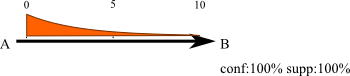
Fig.3 : Example of rule with non-uniform probability distribution for the head. The distribution of this rule is an exponential decay.
Finally, TITARL rules can express complex conditions over time series:
Rule 10: If there is an event A at time t, and if the value of the time series E at time t is lower than five time the value of the time series F, then there is 50% chance to have an event of time B between t + 5 and t + 6.
The last important aspect about TITARL rules is the support. The support of a rule A[t] → B[t+5] 50% is the percentage of event of type B that can be explained by this rule. The support is different from the confidence (actually, the support can be seen as the reverse of the confidence).
Suppose the rule A[t] → B[t+5] 50%.
This rule tells you that when there is an event of type A, there is 50% change to be an event of type B five
seconds later.
Now, suppose that only 10% of events B are preceded by events of type A.
This mean that this rule cannot predict all the events B!
Actually, this rule will only predict 10% of the event B.
This is what is called the support: The support of this rule is 10%.
A rule is interesting if it has a high confidence, a high support, and a high temporal accuracy. When the TITARL algorithm is applied to a symbolic time sequence, the algorithm is able to extract TITARL rules. The next sections explains how the TITARL algorithm is able to do that.
3. The TITARL algorithm
The TITARL algorithm is divided into four main steps. Those steps are :
- The creation of simple unit rules (A unit rule is a rule with only one condition such as A[t] → B[t+5] 50%).
- The division of rules (i.e. splitting a rule into several "smaller" rules)
- The refinement of rules (i.e. polishing the rule to make it slightly better)
- And finally, the addition of a condition to an already existing rule. (i.e. making the rules more complex but more confident)
In the TITARL algorithm, the first step (creation of simple unit rules) is applied once at the beginning. This step returns a set of rule. Then, The three other steps are applied sequentially until the algorithm judges it can stop. The next sections explains each of those steps as well as why they are necessary. The give explanations include some interactive figures that you can play with in order to understand the algorithm.
3.1 The creation of simple unit rules
To create all the initial units rules, the TITARL algorithm starts to list all the possible types of events. Those types of events are depended to the symbolic time sequence on which the TITARL algorithm is applied. For the sake of simplicity, we will call those type of events E1, E2, E3, ..., En (there are n types of events). Once those type of events are listed, the algorithm will create a rule for each pair (Ei,Ej) : Ei[t] → Ej[t-∞,t+∞]. This rule means that if there is an event of type Ei at time t, then there will be an event of type Ej from t-∞ until t+∞.
Since there are n types of events, there is only n x n = n� rules to create. The rules Ei[t] → Ej[t-∞,t+∞] are able to correlate any event that ever existed with any other events that ever existed. If you want to use the TITARL rules to make forecasting prediction, you probably only want to correlate events from the past to the future. Therefore, instead of creating rules like Ei[t] → Ej[t-∞,t+∞], you will configure the the algorithm to only create rules like Ei[t] → Ej[t+0,t+∞] (notice the t+0 instead of the t+∞). Also, since related events are generally temporally close, you might want to tell the algorithm not to look for events which are too far apart! Therefore, instead of creating rules like Ei[t] → Ej[t-0,t+∞], you will configure the algorithm to only create rules like Ei[t] → Ej[t+0,t+h]. In this case, it is up to you to select the value of h. If you don't know what to take for h, simply start by giving it a very large value.
At this point, you will get different rules with different support and confidence. Those rules are simple, and because there are simple, they might not be very good. It is the role of the three other steps to improve them.
Before presenting the other steps, you can notice that some of the rules have confidence or a support so low that they are useless. The next steps will improve their confidence, but they will not be able to improve they support. Therefore, at this point, the algorithm removes all the rules with a low support. It is up to you to chose the minimum support. Generally, I set the minimum support to 5%, and we eventually change it depending on the results.
3.2 The division of a rule
Suppose you are living in a county when it is raining from time to time (At least of couple of time every years -- so not in the Sahara desert for example). Also, suppose that you apply the TITARL algorithm to forcast the next time it will rain. If the algorithm tells you that it will rain in the next ten years, you might not find this information very useful: To be useful, rules needs to be temporally accurate! Therefore we need a way to increase the temporally accuracy of the rules.
At this point, there are up to n� units rules (we have removed the rules with low support), and the temporal accuracy of those rules are very bad. This is true because h (that you defined in the previous step) is very large. This step (the division of a rule) will improve the temporal accuracy of the rules.
The temporal accuracy of a rule is a problem that all temporal data mining techniques are facing. Some techniques simply ignore this problem: Those techniques just ask to the user to select a small value for h. Fortunately, some other techniques are more clever. When facing a rule like Ei[t] → Ej[t-0,t+∞], most techniques are relying of the density distribution between the times of Ei and the time of Ej. More exactly, those techniques are analysing the density distribution P( t - t' | Ei[t] and Ej[t']). Unfortunately, those solutions only work in sparse datasets (by opposition to dense datasets). To illustrate this problem, consider the following example:
Suppose the algorithm to have the rule Ei[t] → Ej[t-0,t+h] (with h very large), and suppose that there is an event Ei at time 1 and two events Ej at time 3 and 4. Should the algorithm try yo explain those two events Ej with the same rule, or should the algorithm try to generate two separated rules like Ei[t] → Ej[t,t+3.5] and Ei[t] → Ej[t+3.5,t+6] to explain the two events independently?
Let's consider another situation: Suppose the algorithm has the rule Ei[t] → Ej[t-0,t+h] (with h very large), and suppose that there are two events Ei at time 1 and 2, and one event Ej at time 5 (This is the opposite of the previous example). Here again, should create two rules or a single one?
Those situations happens when the dataset is dense i.e. when a single rule or when several rules are interlaced. Unfortunately, the density distribution (that we were talking about before) cannot always be use to solve those problem. The figure 3 is an interactive plug-in that illustrates this example. In this figure, you can define one or two rules (that the algorithm does not know about), and see the density distribution of the rule that is being analyzed by the learning algorithm (in the plug-in, h=20 is selected to be small enough to make the example easy to understand).
In the following plug-in, you can define two unit rules. Those rules are hidden from the TITARL algorithm. If you only want to define one rule, you can set the confidence of one of the rule to 0%. Four parameters can be defined for both rules: The left side of the head constraint, the right side of the head constraint, the confidence of the rule and the distribution of the head constraint. The "Snap-shop of events" shows a sample of the randomly generated dataset. This dataset is generated such as the two hidden rules are true. You can use your mouse to navigate in the dataset. "Rule to divide" shows the rule that the TITARL algorithm currently knows. This rule is equivalent of what the algorithm would know after the first step of the algorithm (The creation of simple unit rules). The "Density distribution of the rule to divide" shows the estimated density of this rule.
With the default parameters, two interlaced rules are defined. You can see that the estimated "Density distribution of the rule to divide" hardly helps to detect the two rules. This density could be interpreted as a single, two or three rules. This plug-in illustrates that separating interlaced rules is hard with only the use of the "Density distribution of the rule to divide".
On the plug-in, you can see several collapsed graph below the "Density distribution of the rule to divide". Those graph will be used in the following parts of the tutorial. I recommend you to open a new page with this tutorial so you can continue to read it, while having the plug-in accessible.
Fig 3: Interactive illustration showing that is the density distribution of rules when the dataset is dense and interlaced.
In order to de-interlace rules (and make them more temporally accurate), the TITARL algorithm uses the co-occurence matrix of the predictions of the rules (instead of the density function). The co-occurence matrix can be seen as a two dimensional histogram, where the diagonal is the density function, and where the non-diagonal cells show the relation between events that are predicted together (i.e. by the same prediction). The equation of the co-occurence matrix is:
With s_x = [ x . h / n , ( x + 1 ) . h / n ]
You can see the co-occurence matrix in the plug-in. In the co-occurence matrix, you can see two "blocs" with the default configuration. Each bloc is due to the interaction of the two rules. While it is hard to distinguish the two rules on the density distribution, you can see those two clear "blocs" on the co-occurence matrix. If there is only one rule (you can try it by assigned a confidence of 0% to one of the rules, and 100% to the other), you will see a cross in the co-occurence matrix. This cross is due to the interlacing of the rule with itself. In the case where there is only one rule, you can make the cross disappear by you increase the duration of the dataset, or if you reduce the number of events of type A.
The TITARL algorithm relies on the co-occurence matrix to divide rules (i.e. to find their best temporal accuracy). More precisely, TITARL has two ways of using the co-occurence matrix. Both ways have advantages and inconvenients. The first ways of doing it is based on graph coloration technique. The second way is based on matrix clustering. Before applying any of those two techniques, TITARL applies two filters on the co-occurence matrix.
The first filter is to compute the co-probability matrix M' out of the co-occurence matrix M. The equation of this matrix is:
The second filter is a Gaussian filter (of Gaussian blur) [see Gaussian blur on Wikipedia]. TITARL computes the smoothed co-probability matrix M'' by applying a Gaussian filter on the co-probability matrix M'. You can see the results of those two filters on the plug-in.
The two methods of rule splitting are presented in the next two sub-sections.
3.2.1 Splitting rules with graph coloring
The first method of TITARL to split rule is to suppose the Co-probability matrix and the Smoothed co-probability matrix to be an Adjacency matrix. An Adjacency matrix is a matrix that define a graph [see Adjacency matrix on Wikipedia]. In other words, TITARL create a graph, where the weight between the node n_i and n_j is equal to M'_{i,j}. You can see this graph in the "Graph" plot of the plug-in. The colors are explained in the next paragraph. In this graph, two connected nodes refers to two intervals of the density function with a strong correlation i.e. if an event if predicted in one of the interval, there is a high probability to have an event predicted by the other interval.
Next, TITARL applies a threshold τ on the weights of the edges: All the edges with a weight smaller than τ are removed. Next, TITARL applies a graph coloration algorithm: A Color (i.e. an index) is assigned to every node. Two connected nodes cannot share the same color. The algorithm tries to assign a color to every node while minimizing the total number of color. You can see this graph and the coloration in the "Graph" plot of the plug-in. The task of such type of color labelling is called "Graph coloring". This problem has been shown to be NP-hard. Several heuristics has been developed. TITARL uses the DSAT algorithm to color the graph nodes [New methods to color the vertices of a graph - Br�laz].
Finally, TITARL creates a new rule for each color. All the nodes with the same color will define the temporal constraint in the head of a rule. You can see different splittings of the rule with different value of τ in the "Coloration clustering" plot of the plug-in.
3.2.1 Splitting rules with matrix clustering
The second method of TITARL to split rules based on a matrix clustering. The distance matrix is defined to be the distance between the columns of the Smoothed co-probability matrix. You can see the distance matrix in the plug-in. TITARL uses the Euclidean distance for this task. Next, a hierarchical clustering is applied to generate groups of columns (i.e. groups of intervals of the density function). The TITARL algorithm creates a new rule for each groups of columns. You can see the clusters in the "Matrix clustering" plot of the plug-in.
3.3 The refinement of rules
The refinement of rules is an optional step that "polishes" rules. In this step, a Gaussian blur and a threshold are applied sequentially on the head condition and body conditions are the rules. This operation tends to improve the quality of the rules.
3.4 The addition of a condition to a rule
The addition of a condition to a rule is the last operation of the TITARL algorithm. In a few words, this operation takes as input a set of rules. Then it selects one rule and one new condition for this rule. Finally, it adds this condition to the selected rule, and returns the result.
TITARL rules can contain several type of conditions:
- The temporal conditions i.e. test of existence of an event in a given range of time (this condition can be positive or negative).
- The simple scalar time series conditions i.e. test on the value of a scalar time series at a given time.
- The complex scalar time series conditions i.e. training of a classifier with the values of all the scalar time series as input (this condition is an extension of the previous type of condition).
The selection of the rule and the condition of this step (addition of a condition to a rule) is based on Entropy gain. The rule and the condition that maximize the entropy gain are selected.
The definition of a temporal conditions needs to include the definition of the temporal constraint. TITARL represents temporal constraints by subsets of ℝ (set of real number). Because the set of subsets of ℝ is infinite, TITARL uses an heuristic to find the temporal constraint with the highest entropy gain. More precisely, TITARL can use two version of this heuristic: The first version (the more general) in unconstrained, while the second version is only able to extract connected set-sets of ℝ (i.e. an interval).
3.4.1 Unconstrained selection of set-sets of ℝ
TITARL reduces the selection of a sub-set of ℝ, to the selection and the union of a sub-set of a finite and disjoint set of sub-sets of ℝ. The finite and disjoint set of sub-sets of ℝ is defined by the user. To make this configuration easy, the user has only to define a grid (or a list of borders). Each cell of the grid will be a sub-sets of ℝ. All those sub-sets are disjoint. The grid is not necessarily uniform. The fig. 4 shows three examples of grid that can be defined by the user.
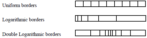
Fig.4 : Example of borders
If the user define a grid will n cells, the TITARL algorithm has to consider 2^n - 1 possible configurations (in order to chose the sub-set of ℝ). Instead, TITARL performs a Gradient descent. The space of the Gradient descent is a binary n dimensional space, where each dimension specify if a particular sub-set of ℝ (a cell in the grid) is selected. In the case of a positive temporal condition, the Gradient descent starts at the coordinate {0}^n. In the case of a negative temporal condition, the Gradient descent starts at the coordinate {1}^n.
3.4.2 Constrained selection of set-sets of ℝ
The difference between the first and second approach is in the selection of a sub-set of cells of the grid. This second approach only selects a connected sub-set of ℝ, which mean that the selected cells should also been connected. If the user define a grid will n cells, the TITARL algorithm has to consider n x ( n + 1 ) / 2 possible configurations. By opposition to the first approach, TITARL will test (efficiently) all those configurations and select the one with the highest entropy gain.